Visualization
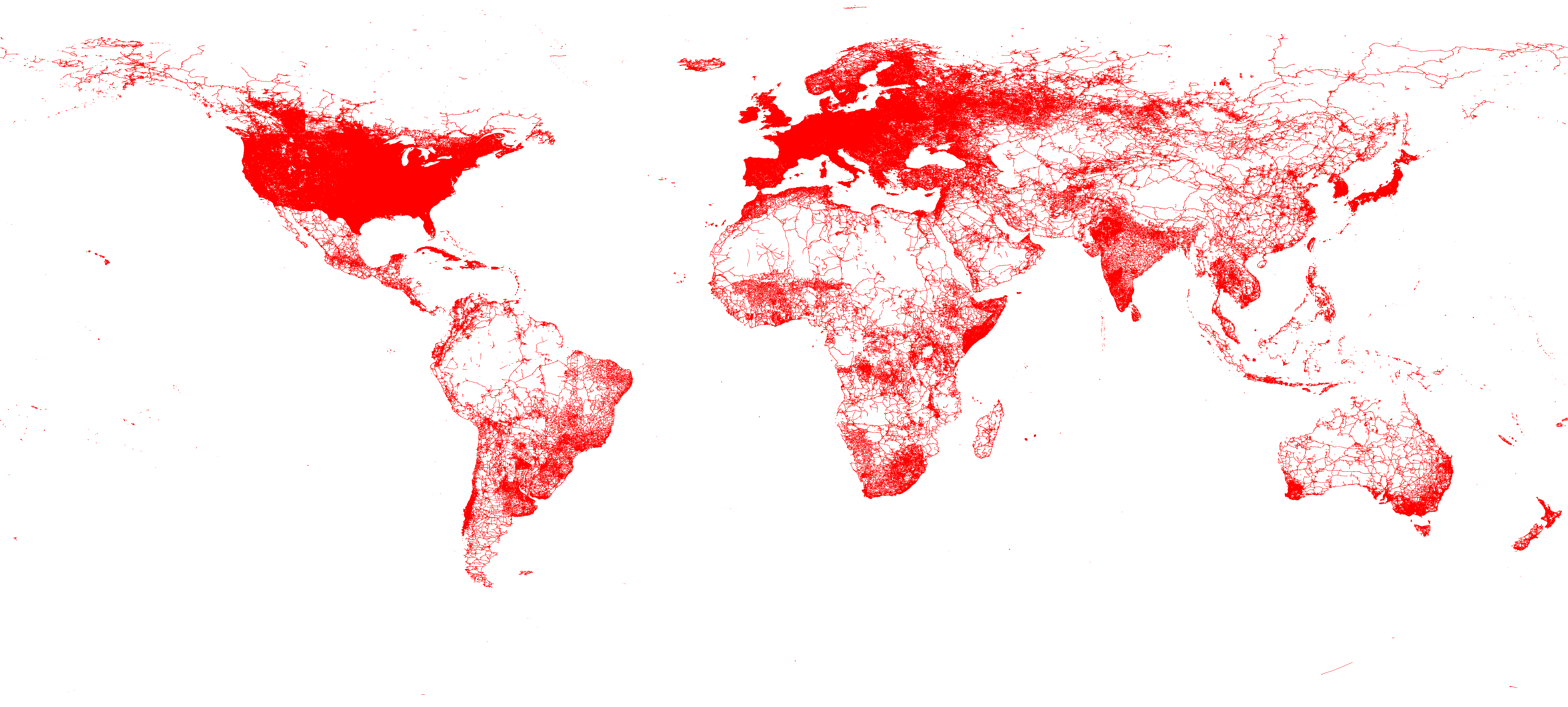
SpatialHadoop provides efficient tools for visualization of large files. This functionality is greatly useful when you have a very large file and you want to get an idea of how the data looks like. For example, the image shown below visualizes all road networks in the globe. This image is created from a dataset of 59 Million lines with a total size of 20.6GB. The dataset is extracted from OpenStreetMap and can be download for free in the datasets page.
SpatialHadoop contains mainly two operations which are responsible of visualization, namely, plot and plotp. plot is used to draw one image at a user specified resolution that summarizes the whole file. plotp is used to draw a pyramid of images at different zoom levels which allows navigation through the image via pan and zoom (similar to Google Maps).
Plot
The command plot is called from the command line. For example, the roads dataset shown above can be visualized using the following command.
$ bin/shadoop plot roads.tsv.bz2 roads.png shape:osm width:2000 height:2000 -keep-ratio color:red -vflip -fast -overwriteThe input file is roads.tsv.bz2. Notice that you do not need to decompress the file. SpatialHadoop will parse the file and decompress it on the fly. The output image will be stored in the file roads.png. shape:osm tells SpatialHadoop that records in the input file are of type osm (i.e., edu.umn.cs.spatialHadoop.core.OSMPolygon). Maximum dimensions of the image is 2000x2000 while keeping the aspect ratio of the input file. To force the output image to be of the given size without respecting the aspect ratio, you can provide the option -no-keep-ratio. color:red tells SpatialHadoop to set the default color to red when drawing lines and points (i.e., vector data). The -vflip option causes the generated image to be vertically flipped. This is useful in this case because the input data has a y-axis (i.e., latitude) that increases from the bottom to the top, while the y-axis on the screen (and image) increases from the top to the bottom. Finally, the -fast tells SpatialHadoop to use a faster method for drawing which does most of the work in the map phase.
When the above command in given to SpatialHadoop, it launches a MapReduce job which plots an image to the given file. In the map function, objects are distributed according to a uniform. Objects overlapping each grid cell are combined together in one reducer which plots all records in that cell to one image. After all reducers are done, one machine stitches all generated images together to produce one image as the output.
Plot Pyramid
The plot command mentioned above is useful to draw an image that summarizes a huge dataset. However, you cannot get any details out of this picture due to the limited resolution of the image and the high level of details in the data. To catch all the details you need to draw a really big picture (say 1M by 1M pixels) which most modern viewers cannot display right. In this case, plotp can be greatly helpful which instead of making one picture, it makes a set of pictures (tiles) at different zoom levels and arranges them in a way that allows navigation in these pictures as if it is one super huge image. The following example shows how to use this command to draw a picture for the roads dataset as shown above.
$ bin/shadoop plotp roads.tsv.bz2 roads shape:osm tile_width:256 tile_height:256 numlevels:8 color:red -vflip -overwriteThe plotp command is very similar to the plot command with two differences. First, instead of width and height, this command uses tile_width and tile_height which specifies the size of each tile used when drawing the picture. The second difference is that you can specify an extra parameter numlevels which specifies the total number of zoom levels to draw. The first level contain one tile of size 256 by 256 pixels (or otherwise specified). The second level contains four images arranged in a 2x2 grid, each image (tile) is of size 256x256. The third level contain tiles arranged in a 4x4 grid, and so on and so forth. In the shown example, the last level contain 256x256 images, each of size 256x256 pixels. This is equivalent to one huge image of size 65,536x65,536 pixels.
The output of this operation is a directory that contains a set of images. In addition, the operation generates an HTML file which uses Google Maps APIs to visualize these images while providing a navigation functionality similar to Google Maps (i.e., pan and zoom).